6 Quality Assurance
In this section, we will show how accurate our translation of the SIMD procedure from SAS to R is. For this, we’ll compare the outputs from SAS and R at different points in the calculation.
You will see that the R code correctly replicates the SAS code, but that there are small numeric differences between SAS and R outputs due to the way SAS and R run the factor analysis procedure, and rounding. This means that SIMD ranks produced through the openSIMD code slightly differ from the official SIMD16 ranks published on the Scottish Government SIMD website.
Future updates of SIMD will be calculated using R, and the openSIMD R code will produce SIMD ranks that are identical with the official SIMD ranks published by the Scottish Government.
6.1 Normalisation
Here, we look at the normalisation step and compare the normalised scores of an education indicator, the percentage of people with no qualifications, calculated in SAS and in R.
Loading the indicator raw data and the (SAS-)normalised indicator scores:
noquals <- read_excel("../openSIMD_analysis/data/SAS NOQUALSDATA.xls")
str(noquals)
## Classes 'tbl_df', 'tbl' and 'data.frame': 6976 obs. of 3 variables:
## $ DZ : chr "S01006506" "S01006507" "S01006508" "S01006509" ...
## $ Noquals : num 52.8 95.9 38.6 80.1 77.2 ...
## $ nnoquals: num -0.7981 0.0512 -1.2185 -0.2042 -0.2607 ...Normalising the indicator data, but now in R:
noquals$r_nnoquals <- normalScores(noquals$Noquals)Comparing the two sets of normalised scores, asking to which degree of precision we have reproduced the result obtained in SAS.
checkEquivalence <- function(x, y, sig_figs) {
  same <- lapply(sig_figs, function(n) identical(signif(x, n), signif(y, n))) %>% unlist
  data.frame(significant_figures = sig_figs, is_identical = same)
}

checkEquivalence(noquals$nnoquals, noquals$r_nnoquals, 1:16)
## significant_figures is_identical
## 1 1 TRUE
## 2 2 TRUE
## 3 3 TRUE
## 4 4 TRUE
## 5 5 TRUE
## 6 6 TRUE
## 7 7 TRUE
## 8 8 TRUE
## 9 9 TRUE
## 10 10 TRUE
## 11 11 TRUE
## 12 12 TRUE
## 13 13 FALSE
## 14 14 FALSE
## 15 15 FALSE
## 16 16 FALSEThe normalised scores for this indicator are identical to eleven decimal places. We believe the remaining differences are due to small differences in how SAS and R work.
6.2 Factor analysis
Here, we look at the factor analysis step.
To test whether SAS and R produce equivalent weights, we load the published indicators and the weights derived from SAS.
indicators <- read_excel("../openSIMD_analysis/data/SIMD16 indicator data.xlsx", sheet = 3, na = "*")
sas_weights <- read_excel("../openSIMD_analysis/data/SAS WEIGHTS.xlsx")
As an example, we’ll calculate the health domain weights.
r_weights <- indicators %>%
  select(CIF, SMR, LBWT, DRUG, ALCOHOL, DEPRESS, EMERG) %>%
  mutate_all(funs(normalScores)) %>%
  mutate_all(funs(replaceMissing)) %>%
  getFAWeights %>%
  unlist
## Warning in qnorm(rn, mean = 0, sd = 1, lower.tail = forwards): NaNs
## produced
## Warning in qnorm(rn, mean = 0, sd = 1, lower.tail = forwards): NaNs
## producedsas_weights <- sas_weights %>% select(wt_cif:wt_emerg) %>% unlist
names(sas_weights) <- NULLNote: You should see a warning here when normalScores propagates a few missing values.
Now that we have the two sets of health domain weights, we can use the same method as above to compare them.
checkEquivalence(sas_weights, r_weights, 1:5)## significant_figures is_identical
## 1 1 TRUE
## 2 2 TRUE
## 3 3 FALSE
## 4 4 FALSE
## 5 5 FALSEThe factor analysis weights are equivalent between the two platforms to two significant figures. Again, we think that this is due to the specific implementation of the factor analysis algorithm in the two platforms.
6.3 Domain ranks
Here, we look at how well domain ranks derived through R correlate with the ranks derived through SAS. First, we need a few more packages, and we will load in the SAS results and R results.
library(tidyr)
library(ggplot2)
library(purrr)
sas_results <- read_excel("../openSIMD_analysis/data/SAS SIMD and domain ranks.xlsx", 1)
r_results <- read.csv("../openSIMD_analysis/results/domain_ranks.csv")
Now we need to select the necessary columns and rename them. Then, we need to join the two datasets together for plotting.
sas_domains <- sas_results %>%
  select(-IZ, -LA, -pop, -wapop, -SIMD)
names(sas_domains) <- c("data_zone", "income", "employment", "health",
                        "education", "access", "crime", "housing")

sas_domains$source <- "sas"
r_results$source <- "r"

sas_domains <- gather(sas_domains, domain, rank, -data_zone, -source)
r_results <- gather(r_results, domain, rank, -data_zone, -source)
results <- rbind(sas_domains, r_results) %>% spread(source, rank)
Finally, we plot the R- and SAS-derived domain ranks against each other and look at the correlations. We also look at the distribution of differences in domain ranks.
ggplot(results, aes(x = sas, y = r)) +
  geom_point() +
  facet_wrap(~ domain)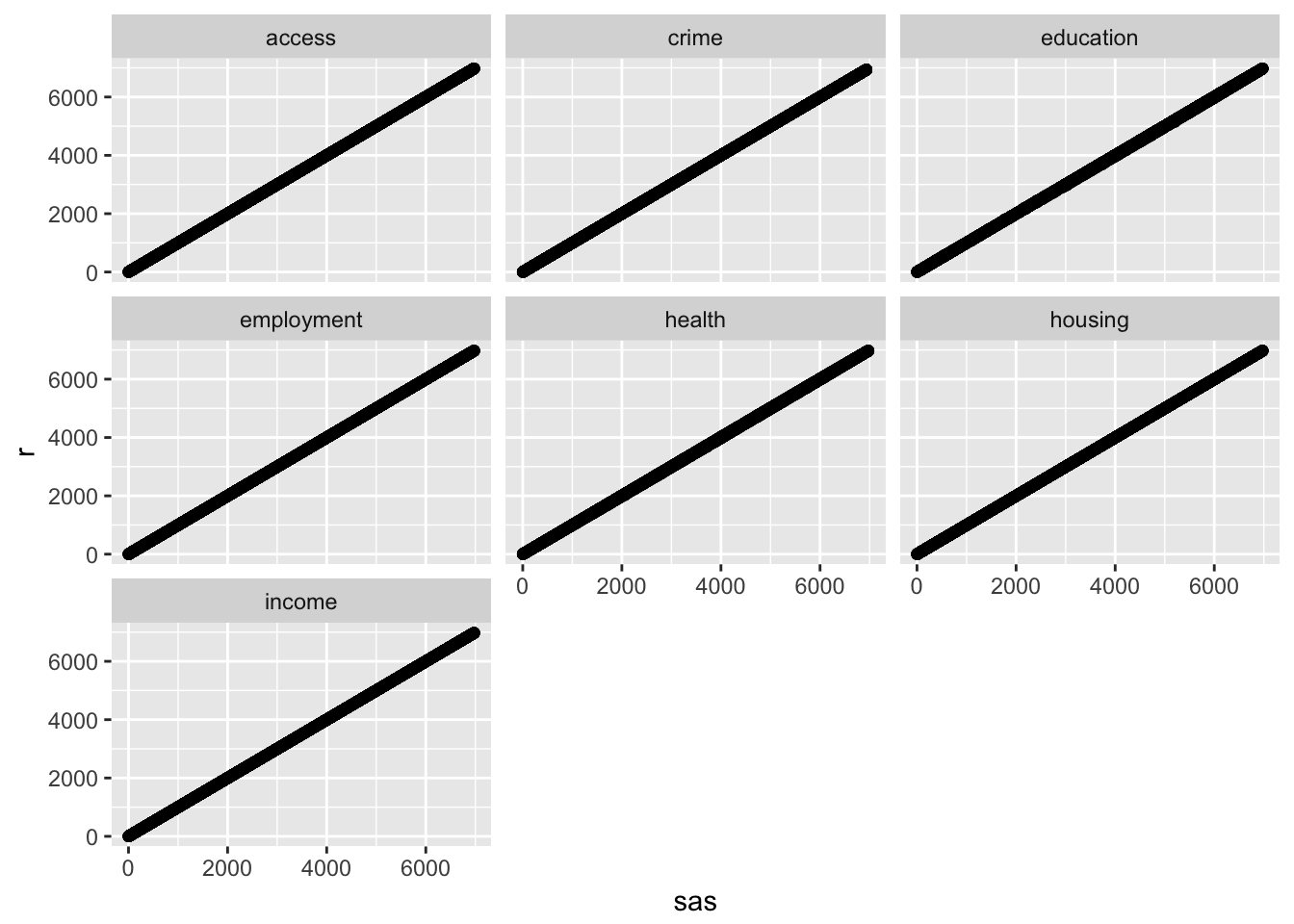
ggplot(results, aes(x = abs(sas - r))) +
  geom_histogram(bins = 20) +
  facet_wrap(~ domain)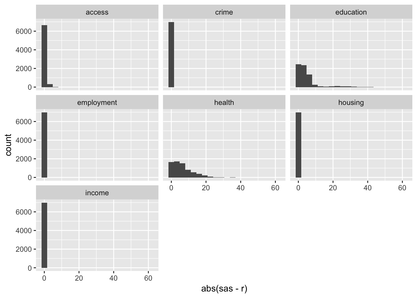
Here, we calculate the correlation coefficient for each comparison, and the median difference in rank.
results %>%
  group_by(domain) %>%
  nest %>%
  mutate(rho = map_dbl(data, ~ cor.test(.$sas, .$r, method = "spearman", exact = FALSE)$estimate)) %>%
  mutate(median_diff = map_dbl(data, ~ median(.$r - .$sas))) %>%
  select(domain, rho, median_diff)
## # A tibble: 7 × 3
## domain rho median_diff
## <chr> <dbl> <dbl>
## 1 access 0.9999999 0
## 2 crime 1.0000000 0
## 3 education 0.9999923 1
## 4 employment 1.0000000 0
## 5 health 0.9999911 0
## 6 housing 1.0000000 0
## 7 income 1.0000000 0The results tell us that the ranks are highly correlated but not exactly equal. The largest rank difference is 61, found in the education domain. These differences are due to the numerical discrepancies in the factor analysis step.
6.4 SIMD ranks
Here, we compare the final SIMD rankings between the two platforms. Again, we need to read in the data and join it up.
sas_simd <- sas_results %>% select(DZ, SIMD)
r_simd <- read.csv("../openSIMD_analysis/results/openSIMD_ranks.csv")
names(sas_simd) <- c("data_zone", "sas")
names(r_simd) <- c("data_zone", "r")
simd_results <- left_join(sas_simd, r_simd)
## Warning in left_join_impl(x, y, by$x, by$y, suffix$x, suffix$y): joining
## factor and character vector, coercing into character vectorThen we examine the correlation in SIMD rankings between R and SAS, and the distribution of differences in SIMD rank.
simd_results %>%
  mutate(rho = cor.test(.$sas, .$r, method = "spearman", exact = FALSE)$estimate) %>%
  mutate(median_diff = median(.$r - .$sas)) %>%
  mutate(domain = 'SIMD') %>%
  select(domain, rho, median_diff) %>%
  slice(1:1)
## # A tibble: 1 × 3
## domain rho median_diff
## <chr> <dbl> <dbl>
## 1 SIMD 0.9999993 0p1 <- ggplot(simd_results, aes(x = sas, y = r)) +
geom_point()
p2 <- ggplot(simd_results, aes(x = abs(sas - r))) +
geom_histogram(bins = 20)
gridExtra::grid.arrange(p1, p2)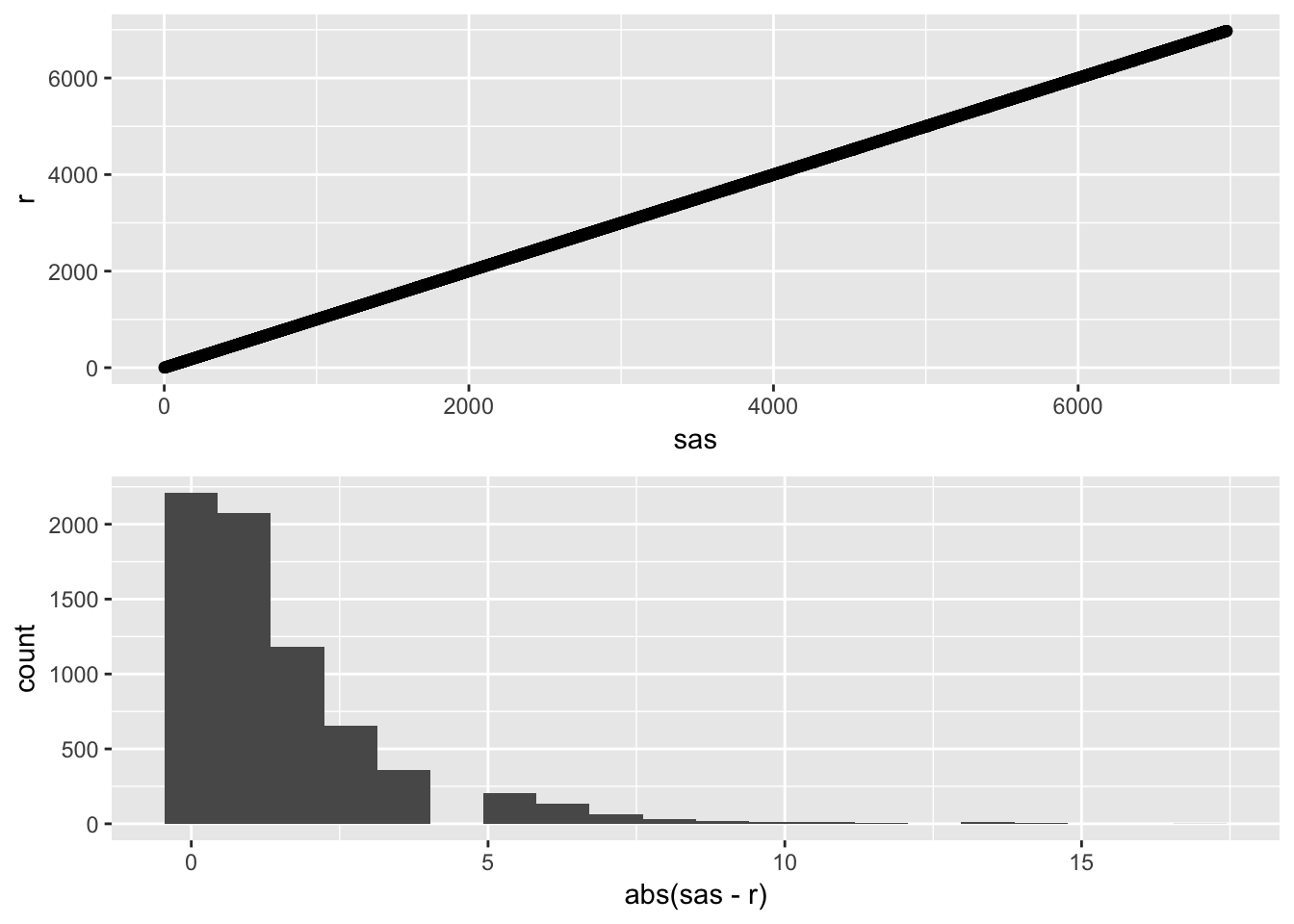
While there is a tight correlation in the final SIMD rankings, there are some differences. Mostly, these differences lie between 0 and 10 with the largest difference as high as 18.
6.5 Conclusion
The differences between rankings derived using R versus using SAS are mainly due to the factor analysis step, which calculates the indicator weights in the health, education, and access domains. As a result, the weights differ in value after the second decimal place. As all discrepancies can be explained, and the correlation is very high, we conclude that the openSIMD R code replicates the original SAS code correctly.